.png)
Spawning biomass (mt)
file: ts7_Spawning_biomass_(mt).png
Spawning biomass (mt)
file: ts7_Spawning_biomass_(mt).png
.png)
Relative spawning biomass: B/(40%*Virgin_Biomass)
file: ts9_Relative_spawning_biomass:_B_per_(40*Virgin_Biomass).png
.png)
Total biomass (mt)
file: ts1_Total_biomass_(mt).png
_at_beginning_of_season_1.png)
Total biomass (mt) at beginning of season 1
file: ts3_Total_biomass_(mt)_at_beginning_of_season_1.png
.png)
Summary biomass (mt)
file: ts4_Summary_biomass_(mt).png
_at_beginning_of_season_1.png)
Summary biomass (mt) at beginning of season 1
file: ts6_Summary_biomass_(mt)_at_beginning_of_season_1.png
.png)
Age-0 recruits (1,000s)
file: ts11_Age-0_recruits_(1000s).png
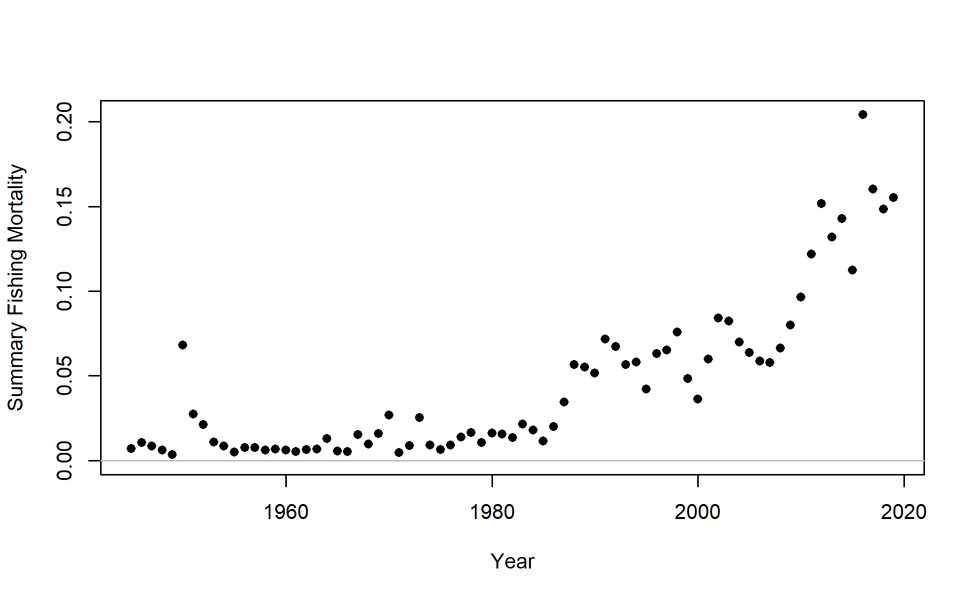
Summary F (definition of F depends on setting in starter.ss)
file: ts_summaryF.png
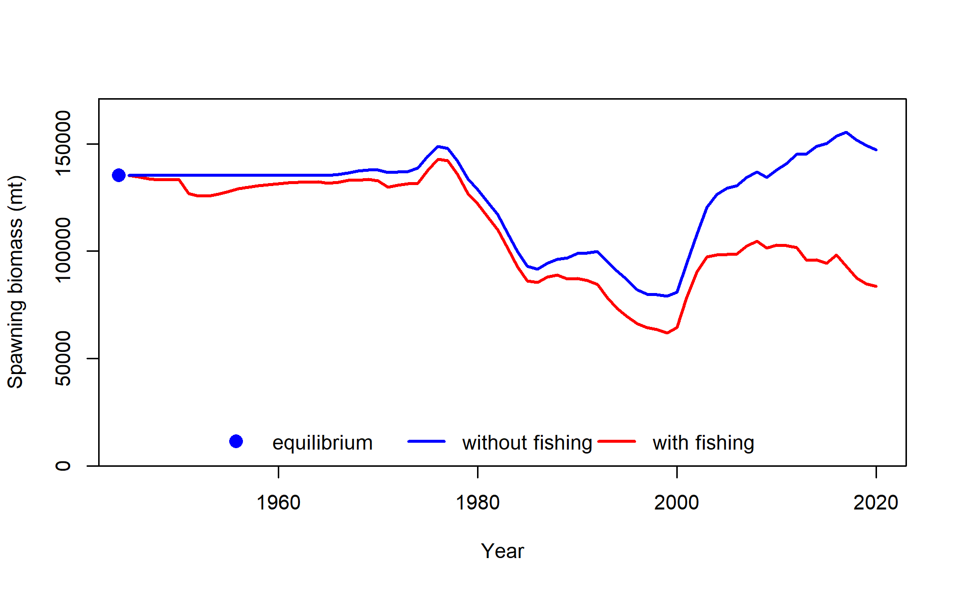
Dynamic B0 plot. The lower line shows the time series of estimated Spawning biomass (mt) in the presence of fishing mortality. The upper line shows the time series that could occur under the same dynamics (including deviations in recruitment), but without fishing. The point at the left represents the unfished equilibrium.
file: ts_DynamicB0.png